class: center, middle, inverse, title-slide # RNA-seq ## Bioformática - LCG-EJ ### Mónica Padilla, Dra. Alejandra Medina ### 2022-03-10 --- # Día 1 **Agenda:** - Presentaciones y Lluvia de Ideas - Overview RNA-seq - Aspectos generales del Pre-Análisis - Diseño Experimental - Diseño de secuenciación - Pipeline bioinformática - Quality Check - Trimming - Ejercicio QC --- # RNA-seq, ¿qué pensamos? .scrollable[ **Actividad:** Lluvia de ideas <img style="border-radius: 90%; width: 150px; top: 1em; right: 1em; position:absolute;" src = "https://media.istockphoto.com/vectors/young-annoyed-female-character-sceptical-face-expression-vector-id1252249414?k=20&m=1252249414&s=612x612&w=0&h=l84MEu6X2KbrRnFbLS2KJ_dswLj0SPIp7pp__cXlRGM="> - Llenen en la siguiente tabla palabras clave sobre RNA-seq: https://docs.google.com/document/d/1pAFddzDlLrRvHMSUjddh7EG3PdTbob3g9UQWzMHXR-w/edit?usp=sharing - Generemos una [figura de nuestras ideas](https://www.r-graph-gallery.com/wordcloud.html): ```r library(wordcloud) library(RColorBrewer) words <- c("Librería,","Secuenciación,","Transcripción,","samtools,","RNA,","","Regulación,","Nucleótido,","Traducción","RNA,","secuenciación,","proteínas,","regulación,","expresión","génica","Secuenciación,","expresión","diferencial,","transcriptoma,","fenotipos","exones","Transcriptoma,","expresión","diferencial,","RNA,","diferencia","celular","Transcripción,","regulación,","expresión,","muestra","Expresion,","exones,","transcriptoma,","UTR,","hisat2,","splicing,","Transcritoma,","splicing,","cDNA") wordcloud(words, colors = RColorBrewer::brewer.pal(5,name = "BuPu")) ``` <!-- --> ] --- # Transcriptómica Estudio del **transcriptoma** - el set completo de transcritos de RNA producidos por el genoma bajo **condiciones específicas** o en una **célula específica** - usando métodos _high-throughput_. - Identidad y abundancia .container[  [4] ] ??? o de alto rendimiento - **¿Por qué la obsesión en el RNA?** Es un intermediario escencial entre el genoma y el proteoma. Entre lo pre-programado y la interacción con el ambiente. --- # ¿Qué es el RNA- seq?  [4] ??? Herramienta que hace uso de las tecnologías de secuenciación NGS para generar perfiles transcriptómicos. --- # Aplicaciones  [5] ??? Responder preguntas biológicas --- # Bases de Datos **Datos de publicación** - NCBI - [Gene Expression Omnibus (GEO)](https://www.ncbi.nlm.nih.gov/geo/browse/) - Sequence Read Archive (SRA) - EMBL-EBI - [ArrayExpress](https://www.ebi.ac.uk/arrayexpress/about.html) **Consorcios ** - [Genotype Tissue-Expression (GTEx)](https://gtexportal.org/home/tissueSummaryPage) - [The Cancer Genome Atlas (TCGA)](https://portal.gdc.cancer.gov/) **Integración de datos para análisis** - [recount3](https://rna.recount.bio/) - [pulmonDB](https://pulmondb.liigh.unam.mx/) --- # Aspectos generales del Pre Análisis ### Diseño Experimental y Diseño de Secuenciación  [1] --- ## Protocolo de extracción de RNA **Propósito:** Deshacerse del RNA ribosomal (90%) y quedarse con el mRNA (~1-2%) .pull-left[ - Eukaryotes - Enriquecer mRNAs usando selección de poly(A) - Degradación mínima del RNA, medido por _RNA Integrity Number (RIN)_ - Prokaryotes o _bad RIN_ - Deshacerse del rRNA] .pull-right[  ] --- ### RNA world - **lncRNA & mRNA**: polyA selection - **miRNA** : binding of 3'UTR target genes - **sncRNA (miRNAs, piRNAs, and endosiRNAs)** : captured by direct ligation with adapters - **circular RNA**: uso de exonuclease R para digerir RNA lineal --- ## Library Type **La mejor opción:** depende del propósito del análisis .pull-left[ - Single-end (SE) - Organismo bien documentado - Bajo costo - Paired-end (PE) reads - Descubrimiento de transcritos _de novo_ - Análisis de expresión de isoformas - Organismo no anotado ] .pull-right[ .fit[  [2] ]] --- ## Sequencing Depth ó Library Size `Número de secuenciación de lecturas para una muestra dada.` **Mejor opción:** depende - 5 millones de lecturas --> Cuantificación adecuada de genes altamente expresados - 100 millones de lecturas --> genes con niveles de expresión bajos En general: `+ sequencing depth = + transcritos + precisión` - Detección de ruido transcripcional ??? curvas de saturacion --- ## Número de replicas Depende de la variabilidad técnica y la variabilidad biológica del objeto de estudio, así como del poder estadístico deseado. .pull-left[ - Variabilidad en mediciones - extracción o _library prep_ - Variabilidad biológica - Inferencias poblacionales: minimo 3 - Poder estadístico - Depende del método] .pull-right[.fit[  [1] ]] --- # Diseño de Secuenciación **Propósito:** Evitar introducir sesgos técnicos o factores de confusión en nuestras muestras. > Nuestro experimento de RNA-seq es grande y las muestras deben de ser procesadas en multiples _batches_ o rondas de secuenciación de Illumina **Aleatorización de muestras** - Durante preparación de librería - Rondas de secuenciación > Muestras individualmente _barcoded_ y se requiren multiples _lanes_ de Illumina para _sequencing depth_ de nuestra elección - Incluir todas las muestras en cada línea para minimizar el _lane effect_ ??? - _spike-ins_ o transcritos exógenos de referencia - QC y normalización --- # Pipeline bioinformática .pull-left[ .container[ ] ] .pull-right[ [4]] --- # Quality Check Some tools: - `FASTQC` Illumina reads - `NGSQC` any platform - `multiqc` : genera reportes gráficos con múltiples muestras Revisar: - Read quality decreases towards the 3' end of reads - Niveles de k-meros, lecturas duplicadas, contenido de GC son experimento y organismo específicos pero deben ser homogeneos --- # Trimming Some tools: `FASTX-Toolkit`, `Trimmomatic`, `cutadapat` Funciones: - Quitar lecturas con mala calidad - Quitar bases con baja calidad - Cortar secuencias de adaptadores --- # Ejercicio QC  --- # References - [1] Conesa, A., Madrigal, P., Tarazona, S., … Mou, S. (2017). RNA-seq methods. Journal of Cellular Biochemistry, 8(1), 1–24. https://doi.org/10.1002/wrna.1364.RNA-Seq - [2] Hrdlickova, R., Toloue, M., & Tian, B. (2017). RNA‐Seq methods for transcriptome analysis. Wiley Interdisciplinary Reviews: RNA, 8(1), e1364. - [3] Stark, R., Grzelak, M., & Hadfield, J. (2019). RNA sequencing: the teenage years. Nature Reviews Genetics, 20(11), 631-656. - [4] Villaseñor-Altamirano, A. B. & Chávez-Domínguez, R. L. "Mini curso abril 2021: Panorama general de análisis de datos de RNA-seq con R". Red Mexicana de Bioinformática (2021). https://comunidadbioinfo.github.io/minicurso_abr_2021/ - [5] Created with BioRender.com --- # Día 2 .scrollable[ **Agenda:** - Caso de estudio, pipeline so far, revisión QC - In-depth Pipeline bioinformática - Alineamiento, Pseudoalineamiento y Conteo - Visualizacion de reads en IGV - Algoritmos de programas famosos - Ejercicio: pseudo-alineamiento con `kallisto` ] ?? ¿Cómo tengo certeza de que mi gen no es un artefacto? --- # Caso de estudio: BRAF inhibition in melanoma cell lines .scrollable[ Número de acceso GEO: [GSE152699](https://www.ncbi.nlm.nih.gov/geo/query/acc.cgi?acc=GSE152699)  _image from (Villaseñor-Altamirano AB, 2021)_ [SRA Run Selector: SRP267712](https://www.ncbi.nlm.nih.gov/Traces/study/?acc=PRJNA640146&o=acc_s%3Aa) :  .red[Nota:] Notemos que cada una de las runs o tandas de secuenciación (identificadas con `SRR`), corresponden a una muestra biológica o réplica (identificadas con `SAMN`). . . . . ] --- # Pipeline so far .scrollable[ ```bash screen -S data qlogin umask 2 # permisos cd mpadilla/clases/rnaseq # change to yours ``` - Obtener archivos fastq - Refs: [fasterq-dump manual](https://github.com/ncbi/sra-tools/wiki/HowTo:-fasterq-dump), [prefetch manual](https://github.com/ncbi/sra-tools/wiki/08.-prefetch-and-fasterq-dump) ```bash module load e-utilities/27abr20 module load sra/2.9.6-1 vdb-config -i # disable storage of cache in ~ mkdir -p data/fastq ``` That opens an interface, press `2` (disable local file caching) > `6` (save) > `7` (exit). ```bash # Get SRR accessions, then download fastq files esearch -db sra -query "SRP267712" | efetch -format docsum | xtract -pattern Runs -ACC @acc -element "&ACC" | xargs fastq-dump --outdir ./data/fastq --gzip --split-3 mv *.fastq.gz data/fastq # move fastq files to their dir esearch -db sra -query "SRP127520" | efetch -format docsum | xtract -pattern Runs -ACC @acc -element "&ACC" | xargs fastq-dump --outdir . --gzip --split-3 ``` - QC current dir = `[mpadilla/clases/rnaseq]` ```bash module load fastqc/0.11.3 fastqc ./data/fastq/*.fastq.gz -o ./out/QC ``` - Trimming Correr iterativamente trimmomatic ```bash mkdir out/trimmed cd out/trimmed module load trimmomatic/0.33 for file in ../../data/fastq/*1.fastq.gz; do trimmomatic PE -phred33 -basein $file -baseout ${file//_1.fastq/_trmd_1.fastq} ILLUMINACLIP:/mnt/Citosina/amedina/mpadilla/resources/trimmomatic/adapters/TruSeq3-PE.fa:2:30:10 SLIDINGWINDOW:5:30 MINLEN:40; done cd ../.. ``` Adapters file downloaded from: https://github.com/timflutre/trimmomatic/blob/master/adapters/TruSeq3-PE.fa, [HiSeq uses TruSeq3 adapters as indicated in trimmomatic manual](http://www.usadellab.org/cms/uploads/supplementary/Trimmomatic/TrimmomaticManual_V0.32.pdf). - QC ```bash mkdir out/QC2 fastqc ./out/trimmed/*.fastq.gz -o ./out/QC2 ``` - Reporte multiqc ```bash module load multiqc/1.5 multiQC ./out/QC2 pwd ``` - See file In local: ```bash rsync -rptuvl mpadilla@dna.liigh.unam.mx:/mnt/Citosina/amedina/mpadilla/clases/rnaseq/out/QC2/multiqc_report.html . # descargar xdg-open multiqc_report.html # abrir archivo ``` ] --- # Pipeline: Dónde estamos .container[  ] --- # Alineamiento  --- # Alineamiento y Conteo ¿Cómo saber qué tipo de algoritmo usar?  --- # Alineamiento con referencia .pull-left[  ] .pull-right[ - ¿Encontrar nuevos transcritos o sólo cuantificar? - PE y alta cobertura - Mapeo singular o múltiple de lecturas - Secuencias repetidas en el genoma, genes paralogos - Mayor mapeo múltiple con transcriptoma debido a isoformas ] --- ### Genoma de referencia  _image from (Villaseñor-Altamirano AB, 2021)_ --- ### Ejemplos genoma de referencia _ _splicing aware__ : Hacen gaps en los reads al compara con el genoma de referencia .container[ ] _image from (Villaseñor-Altamirano AB, 2021)_ ---  --- ### Ejemplo transcriptoma de referencia Programa `kallisto` - Precisos al caracterizar transcritos con alta abundancia, menos precisos con transcritos con menos o cortos .fit[ ] --- # Ensamblaje de novo .pull-left[ - Uso de PE o lecturas largas - Balance en cobertura - Transcritos de baja expresión: unreliable - Mucha cobertura: potencial ensamblaje erróneo y mayor tiempo de ejecución - Combinar reads de todas las muestras para el ensamblaje --> comparaciones adecuadas ] .pull-right[ .container2[  ]] --- # Cuantificación de transcritos .scrollable[ - Enfoque simple: número de reads que mapearon a cada secuencia - `HTSeq-count`, `featureCounts` - Gene-level => gene transfer format (GTF) - `Cufflinks`: PE, GTF o no, toma en cuenta sesgos de longitud de genes, distribución de reads - `sailfish` : k-meros de reads - ¿Cómo sé que mis cuentas corresponden a genes/transcritos? - Referencia con anotaciones - [GENCODE](https://www.gencodegenes.org/mouse/) - [Ensembl](https://www.ensembl.org/info/data/ftp/index.html) `output` : **Cuentas crudas** o _raw counts_ ¿Ya puedo comparar mis niveles de expresión en mi experimento? ] --- # Ejercicio: .scrollable[ ### Alineamiento y conteo usando [`kallisto`][kallisto] .red[ Nota:] cualquier línea de código encerrada en `[]` es opcional o debe cambiarse para tus paths o caso especfíco. Ir a mi directorio en el cluster: ```bash ssh -Y mpadilla@[direccion] cd [/path/a/mi/dir]/mpadilla/ # ir al directorio del proyecto o la clase cd [clases/rnaseq/] ``` Descargar [transcriptoma de referencia de ratón de GENCODE](https://www.gencodegenes.org/mouse/): ```bash mkdir resources; cd resources wget https://ftp.ebi.ac.uk/pub/databases/gencode/Gencode_mouse/release_M28/gencode.vM28.transcripts.fa.gz cd .. # regresar a rnaseq ``` Hacer índice del transcriptoma de referencia que hicimos con GENCODE: - Ver ayuda en [manual de kallisto][kallisto] o en terminal ( `kallisto index -h` ) ```bash module load kallisto/0.45.0 # cargar modulo de kallisto kallisto index -i index_kallisto45_gencode-m28s gencode.vM28.transcripts.fa.gz cd .. # salimos del dir resources ``` * `-i` nombre de archivo de salida, i.e., indice Hacer liga blanda a archivos fastq ya corregidos con trimming: ```bash #ln -rs /mnt/Citosina/amedina/mpadilla/clases/rnaseq/out/trimmed [path/a/tu/dir/]out/ ``` * .red[_Nota:_ ]en clase vimos que no podemos hacer esto si no tenemos permisos. Los datos se copiaron a `/mnt/Timina/bioinfoII/rnaseq/trimmed` Hacer el conteo de transcritos ocupando el índice que hicimos: ```bash mkdir out/kallisto # usar -p si no existe out aun *kallisto quant -i ./resources/index_kallisto45_gencode-m28 -o ./out/kallisto /mnt/Timina/bioinfoII/rnaseq/trimmed/* # once per sample!! ``` * `-o` dir donde colocar output de kallisto - .red[La última línea está mal!] Ahí le estamos diciendo a `kallisto quant` que haga la cuantificación de transcritos con TODOS los archivos fastq, i.e. de todas las muestras juntas, por lo que las cuentas de controles y casos (M14 con BRAF ihnibido o no) estarán combinadas y no podremos hacer comparaciones Para correr `kallisto quant` POR muestra (`SAMN`, recordemos que en este caso cada run `SRR*.fastq` corresponde a una muestra), hagamos lo siguiente: ```bash cd out/kallisto # 1. Hacer dirs de salida para kallisto por muestra: ls ../trimmed/ | perl -pe 's/(SRR\d+)_trmd.*/mkdir $1/' | uniq # copiar texto y pegar en terminal ``` ``` mkdir SRR12038081 mkdir SRR12038082 mkdir SRR12038083 mkdir SRR12038084 mkdir SRR12038085 mkdir SRR12038086 ``` * `ls ../trimmed/` : vemos archivos fastq, identificados por SRR * `perl -pe 's/[match]/[substitution]/'` : con este formato llamamos a perl, `-pe` le dice que corra el siguiente código tomando como input cada línea del STDIN, `s/[match]/[substitution]/` denotamos una subtitución usando expresiones regulares, `(SRR\d+)_trmd.*` guardamos los ids con `()` y seleccionamos el resto, substituimos el texto por `mkdir $1` donde $1 es la variable que guardamos ```bash # 2. Generar lineas para correr kallisto por muestra, ocupando el id SRR como identificador de archivos fastq y dirs ls | grep "SRR" | perl -pe 's/(SRR\d+)/kallisto quant -i ..\/..\/resources\/index_kallisto45_gencode-m28 -o .\/$1 ..\/trimmed\/$1* /' # cambiar archivo en -i por el path a tu indice ``` ``` kallisto quant -i ../../resources/index_kallisto45_gencode-m28 -o ./SRR12038081 ../trimmed/SRR12038081* kallisto quant -i ../../resources/index_kallisto45_gencode-m28 -o ./SRR12038082 ../trimmed/SRR12038082* kallisto quant -i ../../resources/index_kallisto45_gencode-m28 -o ./SRR12038083 ../trimmed/SRR12038083* kallisto quant -i ../../resources/index_kallisto45_gencode-m28 -o ./SRR12038084 ../trimmed/SRR12038084* kallisto quant -i ../../resources/index_kallisto45_gencode-m28 -o ./SRR12038085 ../trimmed/SRR12038085* kallisto quant -i ../../resources/index_kallisto45_gencode-m28 -o ./SRR12038086 ../trimmed/SRR12038086* ``` * `grep` selecciona lineas de STDIN o texto que hagan match * con perl escribimos las lineas para correr kallisto usando el string de las SRR ids al que hicimos match * `../trimmed/SRR12038081*` esta parte tomará las reads a las que hicimos trimmming; como los datos provienen de PAIRED END, son un fastq por cada end (`SRR_trmd_1.fastq` y `SRR_trmd_2.fastq`). _Nota:_ Otra manera de lidear con múltiples archivos, que generen múltiples archivos de salida y que necesitamos para correr en una pipeline es usando `snakemake` o `makefiles` en `bash` Pegar ese output siguiente al sge (`[quant.sge]`) y hacer `qsub quant.sge` ```bash #!/bin/bash # Use current working directory #$ -cwd # # Join stdout and stderr #$ -j y # # Run job through bash shell #$ -S /bin/bash # #You can edit the scriptsince this line # # Your job name *#$ -N [quant] # cambiar # # Send an email after the job has finished #$ -m e *#$ -M [yourmail] # # # If modules are needed, source modules environment (Do not delete the next line): . /etc/profile.d/modules.sh # # Add any modules you might require: *module load kallisto/0.45.0 # # Write your commands in the next line kallisto quant -i index_kallisto45_gencode-m28 -o ./SRR12038081 ../trimmed/SRR12038081* kallisto quant -i index_kallisto45_gencode-m28 -o ./SRR12038082 ../trimmed/SRR12038082* kallisto quant -i index_kallisto45_gencode-m28 -o ./SRR12038083 ../trimmed/SRR12038083* kallisto quant -i index_kallisto45_gencode-m28 -o ./SRR12038084 ../trimmed/SRR12038084* kallisto quant -i index_kallisto45_gencode-m28 -o ./SRR12038085 ../trimmed/SRR12038085* kallisto quant -i index_kallisto45_gencode-m28 -o ./SRR12038086 ../trimmed/SRR12038086* ```  ] --- # Referencias - Grigore, F., Yang, H., Hanson, N. D., VanBrocklin, M. W., Sarver, A. L., & Robinson, J. P. (2020). BRAF inhibition in melanoma is associated with the dysregulation of histone methylation and histone methyltransferases. Neoplasia, 22(9), 376-389. - Conesa, A., Madrigal, P., Tarazona, S., … Mou, S. (2017). RNA-seq methods. Journal of Cellular Biochemistry, 8(1), 1–24. https://doi.org/10.1002/wrna.1364.RNA-SeqConesa, A., Madrigal, P., Tarazona, S., … Mou, S. (2017). RNA-seq methods. Journal of Cellular Biochemistry, 8(1), 1–24. https://doi.org/10.1002/wrna.1364.RNA-Seq - NL Bray, H Pimentel, P Melsted and L Pachter, Near optimal probabilistic RNA-seq quantification, Nature Biotechnology 34, p 525--527 (2016). --- # Día 3 **Agenda:** - Pipeline: Dónde estamos - Importación e integración de datos - Ejercicio - Normalización - Corrección de _batches_ - Exploración de datos con PCA --- # Preguntas - The GFF3 (General Feature Format) format consists of one line per feature, each containing 9 columns of data . [see more](http://www.ensembl.org/info/website/upload/gff3.html) - The GTF (General Transfer Format) is identical to GFF version 2. [see more](http://www.ensembl.org/info/website/upload/gff.html) - GitHub Max Storage (FREE) : 2GB .container[  ] --- # Pipeline: Dónde estamos .scrollable[  _modified from (Villaseñor-Altamirano AB, 2021)_ Nuestro proyecto se ve algo así hasta ahora:  Ver archivo: ```bash cd /mnt/Timina/bioinfoii/rnaseq less out/kallisto/SRR12038081/abundance.tsv ``` ] ??? * `abundances.h5` is a HDF5 binary file containing run info, abundance esimates, bootstrap estimates, and transcript length information length. * `abundances.tsv` is a plaintext file of the abundance estimates. It does not contains bootstrap estimates. The first line contains a header for each column, including estimated counts, TPM, effective length. + `target_id` = transcript id, cambia dependiendo del archivo de anotacion + `length` + `eff_length` = effective length + `est_counts` = estimated counts + `tpm` = Transcripts per million (TPM) is a measurement of the proportion of transcripts in your pool of RNA. * `run_info.json` is a json file containing information about the run. We can facilitate further work by saving this files in a dir with the SRA ID name. --- # Importación e Integración de datos .scrollable[  Paquetes bioconductor: `tximeta` y [`tximport`](https://bioconductor.org/packages/devel/bioc/vignettes/tximport/inst/doc/tximport.html)  ] --- # Ejercicio .scrollable[ **Summarizing to gene level from transcript abundance with `tximport`** ```bash screen -S txi qlogin cd [su/path/en/cluster] cd out/kallisto/ module load r/4.0.2 R ``` En R: ```r library(tximport) library(tidyverse) # stringr # Load data files <- file.path("/mnt/Timina/bioinfoII/rnaseq/out/kallisto",list.dirs(dir2counts),"abundance.h5") # abundance files paths names(files) <- str_extract(files,"SRR\\d+") # so that tximport identifies them files ``` ``` SRR12038081 "/mnt/Timina/bioinfoII/rnaseq/out/kallisto/SRR12038081/abundance.h5" SRR12038082 "/mnt/Timina/bioinfoII/rnaseq/out/kallisto/SRR12038082/abundance.h5" SRR12038083 "/mnt/Timina/bioinfoII/rnaseq/out/kallisto/SRR12038083/abundance.h5" SRR12038084 "/mnt/Timina/bioinfoII/rnaseq/out/kallisto/SRR12038084/abundance.h5" SRR12038085 "/mnt/Timina/bioinfoII/rnaseq/out/kallisto/SRR12038085/abundance.h5" SRR12038086 "/mnt/Timina/bioinfoII/rnaseq/out/kallisto/SRR12038086/abundance.h5" ``` ```r # Load table with trx id and gene id corrspondence tx2gene <- read.csv("/mnt/Timina/bioinfoII/rnaseq/resources/gencode/gencode.v38.basic.pc.transcripts.enstid_ensgid-nover.csv",stringsAsFactors = F) # Load table with trx id and gene name corrspondence tx2genename <- read.csv("/mnt/Timina/bioinfoII/rnaseq/resources/gencode/gencode.v38.basic.pc.transcripts.enstid_genename-nover.csv",stringsAsFactors = F) # Run tximport # tx2gene links transcript IDs to gene IDs for summarization txi.kallisto <- tximport(files, type = "kallisto", tx2gene = tx2gene, ignoreAfterBar=TRUE, ignoreTxVersion=TRUE) txi.kallisto.name <- tximport(files, type = "kallisto", tx2gene = tx2genename, ignoreAfterBar=TRUE, ignoreTxVersion=TRUE) ``` ``` 1 2 3 4 5 6 removing duplicated transcript rows from tx2gene transcripts missing from tx2gene: 92813 summarizing abundance summarizing counts summarizing length ``` ```r names(txi.kallisto) ``` ``` [1] "abundance" "counts" "length" [4] "countsFromAbundance" ``` ```r head(txi.kallisto$counts) ``` ``` SRR12038081 SRR12038082 SRR12038083 SRR12038084 SRR12038085 ENSMUSG00000000001 130.00000 73.00000 53.00000 60 96.000000 ENSMUSG00000000056 0.00000 0.00000 0.00000 0 0.000000 ENSMUSG00000000058 2.00000 1.00000 2.00000 2 4.000000 ENSMUSG00000000078 13.58842 13.58842 12.22958 9 4.076527 ENSMUSG00000000088 81.00000 43.00000 38.00000 31 47.000000 ENSMUSG00000000093 15.00000 11.00000 8.00000 7 12.000000 SRR12038086 ENSMUSG00000000001 98.00000 ENSMUSG00000000056 0.00000 ENSMUSG00000000058 0.00000 ENSMUSG00000000078 5.43537 ENSMUSG00000000088 70.00000 ENSMUSG00000000093 15.00000 ``` transcript estimation --> read counts ] --- # Normalización ### ¿Por qué es necesario normalizar? Nuestros datos están sujetos a **sesgos técnicos y biológicos** que provocan variabilidad en las cuentas. Si queremos hacer **comparaciones de niveles de expresión entre muestras** es necesario ajustar los datos tomando en cuenta estos sesgos. - Análisis de expresión diferencial - Visualización de datos - en general, siempre que estemos comparando expresión ### ¿Qué es normalizar en sí? El proceso de ajuste de las cuentas (scaling factors) por los sesgos "no interesantes" de varibialidad. ??? Comparar niveles de expresión entre genes y entre muestras. - Las cuentras crudas no son adecuadas para comparar entre muestras - Gene/transcript length - Número total de reads - Sesgos de secuenciación - Normalización _within-sample_ - Tamaño de librería: Número de secuenciación de lecturas para una muestra dada --- ## Criterios o sesgos a considerar - Pueden ser relevantes para la comparacion de la expresión .red[entre muestras distintas] (eg muestra control vs muestra caso) y/o .red[dentro de una misma muestra] muestras (entre genes). - __Sequencing depth__ : En este caso, cada gen parece expresarse el doble cuando comparamos `Sample A` vs `Sample B`, sin embargo, sólo parece a sí porque la `Sample A` tuvo el doble de secuenciación - .red[entre muestras distintas] .fit[  ] --- ## Criterios o sesgos a considerar - __Sequencing depth__ - **Método:** Dividir por el size factor  --- ## Criterios o sesgos a considerar .pull-left[ - __Gene length__ : El `Gene X` y el `Gene Y` tienen tienen niveles similares de expresión pero el número de lecturas mapeadas será mayor en el `Gen X` porque es más largo. - .red[misma muestra] - Método: dividir por el largo del gen ] .pull-right[ .fit[  ] ] --- ## Criterios o sesgos a considerar .pull-left[ - __Composición de RNA__ : Si normalizamos dividiendo las cuentas entre el numero total de cuentas en cada muestra, el resto de los genes en la Sample A se verán ampliamente afectados por el Gene DE - .red[entre muestras distintas] - Genes altamente diferencialmente expresados - Diferencias en el número de genes expresados -- PCR - Contaminación ] .pull-right[.fit[ ] ] --- .scrollable[ 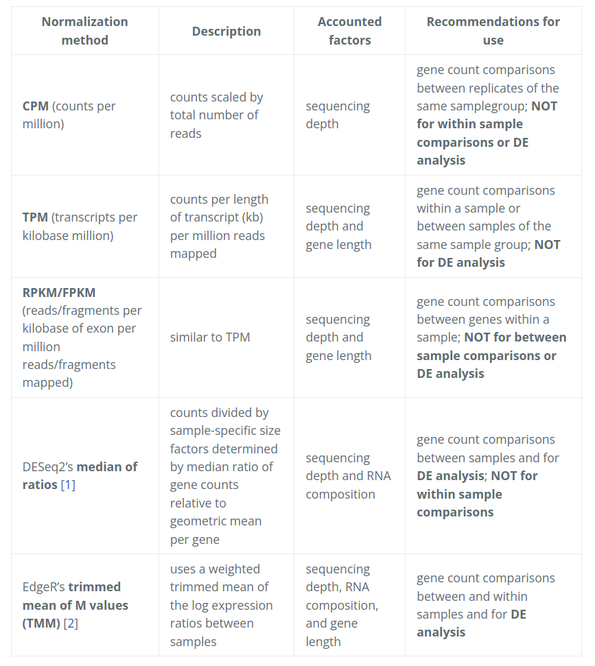] --- # Corrección por _batch effect_ **Mal diseño experimental ==> Mucho _batch effect_** - En este caso no se podría tener certeza sobre ningún resultado 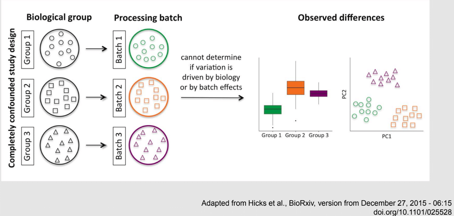 --- ## Corrección por _batch effect_ **Buen diseño experimental, pero aun puede haber variación técnica** 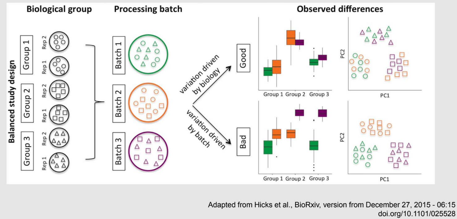 --- ## Corrección por _batch effect_ ¡Pero no todo está perdido! 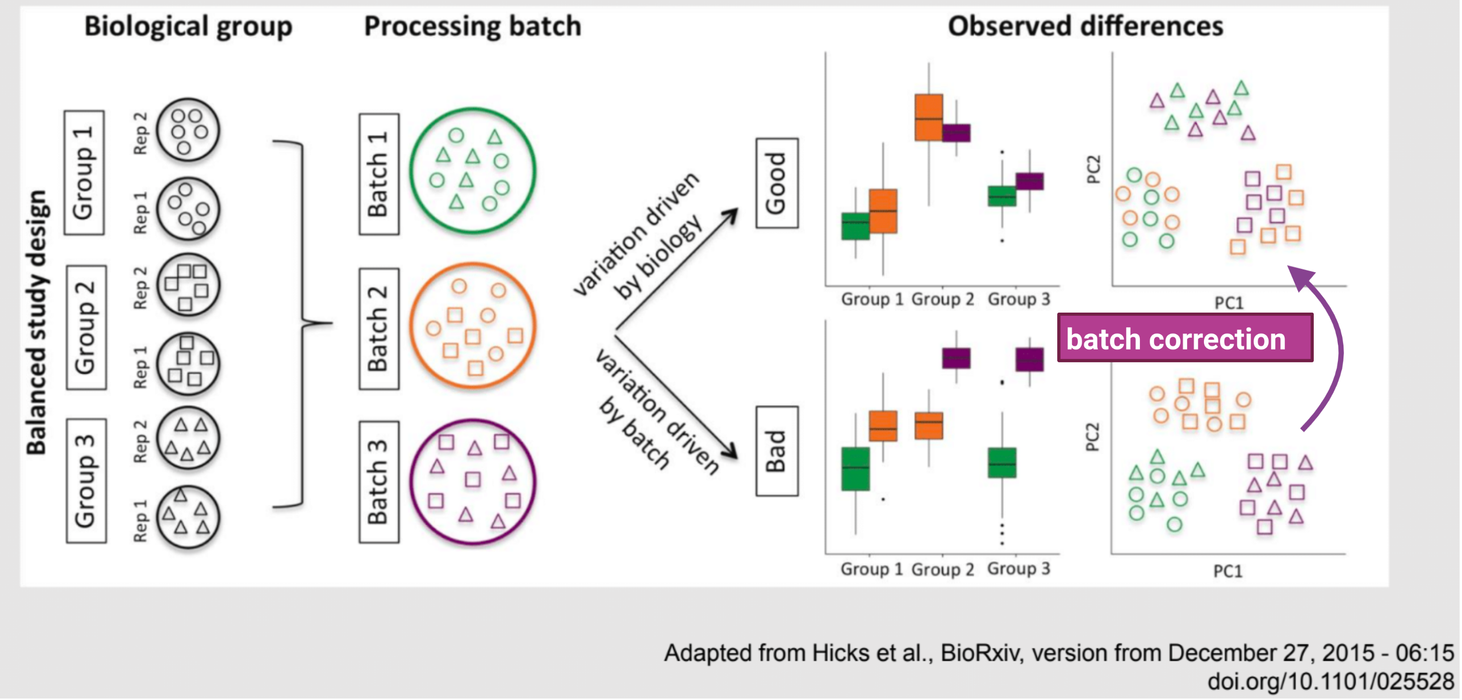 --- # Métodos de ajuste para RNA-seq .scrollable[ - `edgeR` - `ComBat -batch` - `ComBat_seq -batch -bio_conditions` : - Supone una binomial negativa  ] --- # Visualización de datos reales  - Balance entre integración de datasets para ganar poder estadístico y la capacidad de los algoritmos por deshacerse del _batch effect_ --- # Referencias - Soneson, C., Love, M. I., & Robinson, M. D. (2015). Differential analyses for RNA-seq: transcript-level estimates improve gene-level inferences. F1000Research, 4. - Meeta Mistry, R. K. (2017, April 26). Count normalization with deseq2. Introduction to DGE - ARCHIVED. Retrieved March 3, 2022, from https://hbctraining.github.io/DGE_workshop/lessons/02_DGE_count_normalization.html - Zhang, Y., Parmigiani, G., & Johnson, W. E. (2020). ComBat-seq: batch effect adjustment for RNA-seq count data. NAR genomics and bioinformatics, 2(3), lqaa078. --- # Día 4 **Agenda:** - Pipeline: Dónde estamos - Ejercicio: Normalización de DESeq2 - Ejercicio: Visualización de datos - Análisis de Expresión Diferencial - Ejercicio con `DESeq2` - Análisis Funcional --- # Pipeline: Dónde estamos .scrollable[  - Leer detalles de experimento - Los programas trabajan con el input que le das ver sge de `kallisto quant`: ```bash less /mnt/Citosina/amedina/mpadilla/clases/rnaseq/out/kallistoh/quant.sge ``` ``` kallisto quant -i /mnt/Citosina/amedina/mpadilla/resources/kallisto/index_kallisto45_gencode38_hsapiens_cds -o ./SRR12038081 ../trimmed/SRR12038081* ``` ] --- # Normalización con DESEq2 .scrollable[ - Normalización para DE: ajuste por - .spoiler[ Composición de RNA y _Sequencing depth_ ] - `DESeq2` ajusta a un modelo lineal generalizado (GLM) de la familia binomial negativa (NB). ``` ## # A tibble: 2 x 3 ## gene muestraA muestraB ## <chr> <dbl> <dbl> ## 1 gene1 1749 943 ## 2 gene2 35 29 ``` - Crea una pseudo-referencia por muestra (promedio geometrico por fila) `\({\bar {x}}={\sqrt[{n}]{\prod _{i=1}^{n}{x_{i}}}}={\sqrt[{n}]{x_{1}\cdot x_{2}\cdots x_{n}}}\)` ``` ## # A tibble: 2 x 4 ## # Rowwise: ## gene muestraA muestraB prom_geom ## <chr> <dbl> <dbl> <dbl> ## 1 gene1 1749 943 1284. ## 2 gene2 35 29 31.9 ``` Se calcula la fracción `\(muestraN/prom-gem\)` ``` ## # A tibble: 2 x 6 ## # Rowwise: ## gene muestraA muestraB prom_geom muestraA_pseudo_ref muestraB_pseudo_ref ## <chr> <dbl> <dbl> <dbl> <dbl> <dbl> ## 1 gene1 1749 943 1284. 1.36 0.734 ## 2 gene2 35 29 31.9 1.10 0.910 ``` Se calcula un factor de normalización (size factor) utilizando la mediana por columnas. ``` ## [1] 1.230235 ## [1] 0.8222689 ``` Se dividen las `\(cuentas-crudas/size-factor\)` para calcular las cuentas normalizadas. ``` ## # A tibble: 2 x 3 ## # Rowwise: ## gene muestraA muestraB ## <chr> <dbl> <dbl> ## 1 gene1 1749 943 ## 2 gene2 35 29 ``` ``` ## # A tibble: 2 x 2 ## # Rowwise: ## norm_muestraA norm_muestraB ## <dbl> <dbl> ## 1 1422. 1147. ## 2 28.4 35.3 ``` _tomado de (Vilaseñor-Altamirano AB, 2021)_ ] --- # Otras transformaciones .scrollable[ Puedes realizar otras transformaciones en `DESeq2` para estabilizar la varianza a través de los differentes valores promedio de expresión. - Variance stabilizing transformation `vst` (n < 30 ) - Regularized-logarithm transformation (rlog) Propósito: visualización  Los genes con menor expresión tienen más varianza.  _Slide tomada de (Villaseñor-Altamirano, 2021)_ ] --- # Análisis de Expresión Diferencial **¿La diferencia de expresión entre controles vs caso es significativa?** .container[  ] --- # Análisis de Expresión Diferencial **¿La diferencia de expresión entre controles vs caso es significativa?** .container[  ] --- # Ejercicio: Normalización y DE con `DESeq2` .scrollable[ - input: un-normalized, count (or estimated count/fragments) data in the form of a matrix of integer values ```r getwd() ``` ``` [1] "/mnt/Citosina/amedina/mpadilla/clases/rnaseq" ``` Generar matriz de cuentas con `tximport` (Vease slide 39) ```r library(tximport) library(tidyverse) # stringr # ajustar esta línea porque estoy parada en otro dir files <- file.path("/mnt/Timina/bioinfoII/rnaseq",list.dirs("out/kallistoh"),"abundance.h5")[-1] names(files) <- str_extract(files,"SRR\\d+") # Load table with trx id and gene id corrspondence tx2gene <- read.csv("/mnt/Timina/bioinfoII/rnaseq/resources/gencode/gencode.v38.basic.pc.transcripts.enstid_ensgid-nover.csv",stringsAsFactors = F) # Generar matriz txi.kallisto <- tximport(files, type = "kallisto", tx2gene = tx2gene, ignoreAfterBar=TRUE, ignoreTxVersion=TRUE) txi.kallisto$counts %>% head ``` ``` SRR12038081 SRR12038082 SRR12038083 SRR12038084 SRR12038085 SRR12038086 KLHL17 2.043531 3 7.724302 16.000000 19.00000 2.995178 NOC2L 249.941470 151 102.790889 251.562665 292.69206 196.903335 OR4F16 0.000000 0 0.000000 0.000000 0.00000 0.000000 OR4F29 0.000000 0 0.000000 0.000000 0.00000 0.000000 OR4F5 0.000000 0 0.000000 0.000000 0.00000 0.000000 SAMD11 0.000000 0 2.158024 2.488777 4.92229 3.585071 ``` DESeq2 requiere conocer cuáles muestras son controles y cuáles son los casos - Añadimos información de nuestro experimento a.k.a. `metadata` ```r samples <- read.csv("/mnt/Timina/bioinfoII/rnaseq/data/metadata/samples.csv",stringsAsFactors = F, header = TRUE) # obtained parsing file on SRA Run Selector samples <- column_to_rownames(samples, var = "sample") samples ``` ``` cell_line genotype org type condition SRR12038081 M14s BRAFV600E Homo_sapiens Melanoma untreated SRR12038082 M14s BRAFV600E Homo_sapiens Melanoma untreated SRR12038083 M14s BRAFV600E Homo_sapiens Melanoma untreated SRR12038084 M14s BRAFV600E Homo_sapiens Melanoma Verafinib SRR12038085 M14s BRAFV600E Homo_sapiens Melanoma Verafinib SRR12038086 M14s BRAFV600E Homo_sapiens Melanoma Verafinib ``` Construir objeto `DESeqDataSet`, definir modelo de DE (especififcar controles y casos) - Datos introducidos como modelo estadístico (formula de diseño) ```r library(DESeq2) dds <- DESeqDataSetFromTximport(txi.kallisto, colData = samples, design = ~ condition) # + si hay vars en condiciones ``` ``` using counts and average transcript lengths from tximport Warning message: In DESeqDataSet(se, design = design, ignoreRank) : some variables in design formula are characters, converting to factors ``` ```r dds ``` ``` class: DESeqDataSet dim: 6 6 metadata(1): version assays(2): counts avgTxLength rownames(6): KLHL17 NOC2L ... OR4F5 SAMD11 rowData names(0): colnames(6): SRR12038081 SRR12038082 ... SRR12038085 SRR12038086 colData names(5): cell_line genotype org type condition ``` Normalización y Expresión Diferencial con `DESeq2` : ```r # Prefiltrado para quitar genes con cuentas bajas keep <- rowSums(counts(dds)) >= 6 dds <- dds[keep, ] dds$condition <- factor(dds$condition, levels = c("untreated","Verafinib")) dds <- DESeq(dds) ``` ``` estimating size factors using 'avgTxLength' from assays(dds), correcting for library size estimating dispersions gene-wise dispersion estimates mean-dispersion relationship final dispersion estimates fitting model and testing ``` ```r # use contrast= parameter if design formula has > 2 levels res <- results(dds) res ``` ``` log2 fold change (MLE): condition untreated vs Verafinib Wald test p-value: condition untreated vs Verafinib DataFrame with 6 rows and 6 columns baseMean log2FoldChange lfcSE stat pvalue padj <numeric> <numeric> <numeric> <numeric> <numeric> <numeric> KLHL17 6.54932 -0.434353 0.686012 -0.633157 0.526631 0.526631 NOC2L 218.40214 0.621498 0.571255 1.087952 0.276616 0.414924 OR4F16 0.00000 NA NA NA NA NA OR4F29 0.00000 NA NA NA NA NA OR4F5 0.00000 NA NA NA NA NA SAMD11 1.88592 -1.534003 1.351734 -1.134841 0.256442 0.414924 ```  ] --- ## Visualización de datos usando `PCA` .container[ ] _imagen tomada de (Villaseñor-Altamirano, 2021)_ --- # Visualización usando Volcano Plots .fit[  ] --- # Análisis Funcional Gene Ontology (GO term) Enrichment Analysis - `EnrichR`, `TopGO`, `Gprofiler`, `GORilla` - Databases - Ejemplo: .container[ ] --- # RNA-seq, ¿qué pensamos ahora? .scrollable[ **Actividad:** Lluvia de ideas <img style="border-radius: 90%; width: 150px; top: 1em; right: 1em; position:absolute;" src = "https://media.istockphoto.com/vectors/young-annoyed-female-character-sceptical-face-expression-vector-id1252249414?k=20&m=1252249414&s=612x612&w=0&h=l84MEu6X2KbrRnFbLS2KJ_dswLj0SPIp7pp__cXlRGM="> - Llenen en la siguiente tabla palabras clave sobre RNA-seq: https://docs.google.com/document/d/1pAFddzDlLrRvHMSUjddh7EG3PdTbob3g9UQWzMHXR-w/edit?usp=sharing - Generemos una [figura de nuestras ideas](https://www.r-graph-gallery.com/wordcloud.html): ```r library(wordcloud) library(RColorBrewer) words <- c("Expresióndiferencial","comparación de medias","sesgos","control de calidad","pipeline ","análisis funcional ExpresiónDiferencial","PCA","Transcripción","Batch effect","Counts.RNA","secuenciación","proteínas","regulación","expresióngénica","expresión diferencial","normalización","sequencing depthTranscriptoma","RNA","expresióndiferencial","conteo","normalización","Volcano plot","batch effect","sesgos","composición de RNA","tamaño del gen","sequencing depth","alineamiento","Expresiondiferencial","pipeline","normalizacion","transcriptoma","matriz de cuentas","size factor","transcritos","algoritmosTranscriptoma","expresión","diferenciación","sesgos","PCA","significancia","normalización","alineamiento","genomade referenciaExpresion","exones","transcriptoma","UTR","hisat2","splicing","DE","normalizacion","volcanoplot","PCA") wordcloud(words, colors = RColorBrewer::brewer.pal(5,name = "BuPu")) ``` <!-- --> ] --- # Referencias http://bioconductor.org/packages/release/workflows/vignettes/rnaseqGene/inst/doc/rnaseqGene.html https://biocorecrg.github.io/CRG_RIntroduction/volcano-plots.html --- # Gracias!  --- # Día 5 **Agenda:** - Revisitar resultados de DEA - MAplot - Volcano plot con ggplot - heatmap - Enriquecimiento funcional de términos GO - Ejercicio con gprofiler --- # Resultados DE .scrollable[ - DESeq2 performs for each gene a hypothesis test to see whether evidence is sufficient to decide against the null hypothesis that there is zero effect of the treatment on the gene and that the observed difference between treatment and control was merely caused by experimental variability (i.e., the type of variability that you can expect between different samples in the same treatment group). ```r res ``` ``` log2 fold change (MLE): condition Verafinib vs untreated Wald test p-value: condition Verafinib vs untreated DataFrame with 12371 rows and 6 columns baseMean log2FoldChange lfcSE stat pvalue <numeric> <numeric> <numeric> <numeric> <numeric> ENSG000000000035 53.15332 -2.328062 1.310704 -1.776192 7.57013e-02 ENSG000000004194 4.51349 1.076738 1.046573 1.028822 3.03563e-01 ENSG000000004574 12.51881 -0.393507 1.191887 -0.330155 7.41283e-01 ENSG000000004607 17.76331 -2.630115 1.230373 -2.137657 3.25446e-02 ENSG000000009716 62.32683 5.396259 0.685695 7.869768 3.55299e-15 ... ... ... ... ... ... ENSG00000288699 6.85454 -2.502914 2.723702 -0.918938 0.3581278 ENSG00000288701 255.71582 0.450524 0.239893 1.878017 0.0603788 ENSG00000288709 1.37077 -0.413138 3.674915 -0.112421 0.9104894 ENSG00000288710 4.21706 1.528236 2.526702 0.604834 0.5452892 ENSG00000288722 13.09369 -0.151997 0.783592 -0.193974 0.8461960 padj <numeric> ENSG000000000035 2.53340e-01 ENSG000000004194 5.69300e-01 ENSG000000004574 8.90212e-01 ENSG000000004607 1.46951e-01 ENSG000000009716 1.12924e-12 ... ... ENSG00000288699 0.625206 ENSG00000288701 0.219065 ENSG00000288709 NA ENSG00000288710 0.768360 ENSG00000288722 0.940957 ``` - column `log2FoldChange` is the effect size estimate. It tells us how much the gene’s expression seems to have changed due to treatment with dexamethasone in comparison to untreated samples - uncertainty associated with it, which is available in the column `lfcSE`, the standard error estimate for the log2 fold change estimate - `p value` indicates the probability that a fold change as strong as the observed one, or even stronger, would be seen under the situation described by the null hypothesis - Now, assume for a moment that the null hypothesis is true for all genes, i.e., no gene is affected by the treatment with dexamethasone. Then, by the definition of the p value, we expect up to 5% of the genes to have a p value below 0.05. - Benjamini-Hochberg (BH) adjustment: calculates for each gene an adjusted p value ```r summary(res) # if we consider a fraction of 10% false positives acceptable, we can consider all genes with an adjusted p value below 10% = 0.1 as significant ``` ```r out of 12371 with nonzero total read count *adjusted p-value < 0.1 LFC > 0 (up) : 944, 7.6% LFC < 0 (down) : 1072, 8.7% outliers [1] : 47, 0.38% low counts [2] : 1200, 9.7% (mean count < 2) [1] see 'cooksCutoff' argument of ?results [2] see 'independentFiltering' argument of ?results ``` Aplicar un filtro más estricto: - Lower the false discovery rate threshold (the threshold on `padj` in the results table) ```r res.05 <- results(dds, alpha = 0.05) table(res.05$padj < 0.05) # genes that rejected null hypothesis ``` ``` FALSE TRUE 9462 1423 ``` ```r summary(res.05) ``` ``` out of 12371 with nonzero total read count adjusted p-value < 0.05 LFC > 0 (up) : 670, 5.4% LFC < 0 (down) : 753, 6.1% outliers [1] : 47, 0.38% low counts [2] : 1439, 12% (mean count < 2) ``` - Raise the log2 fold change threshold from 0 using the `lfcThreshold` argument of results - test for genes that show more substantial changes due to treatment - `lfcThreshold = 1`, we test for genes that show significant effects of treatment on gene counts more than doubling or less than halving, because 2^1=2 ```r resLFC1 <- results(dds, lfcThreshold=1) table(resLFC1$padj < 0.1) ``` ``` FALSE TRUE 10284 361 ``` ```r summary(resLFC1) ``` ``` out of 12371 with nonzero total read count adjusted p-value < 0.1 LFC > 1.00 (up) : 181, 1.5% LFC < -1.00 (down) : 180, 1.5% outliers [1] : 47, 0.38% low counts [2] : 1679, 14% (mean count < 3) [1] see 'cooksCutoff' argument of ?results [2] see 'independentFiltering' argument of ?results ``` Aplicar filtro `padj < 0.1` en el dataset: ```r resSig <- subset(res, padj < 0.1) # subset head(resSig[ order(resSig$log2FoldChange), ]) # more downregulated genes ``` ``` log2 fold change (MLE): condition Verafinib vs untreated Wald test p-value: condition Verafinib vs untreated DataFrame with 6 rows and 6 columns baseMean log2FoldChange lfcSE stat pvalue <numeric> <numeric> <numeric> <numeric> <numeric> ENSG000001700062 599.8734 -10.88831 2.03420 -5.35264 8.66813e-08 ENSG000001783812 104.3246 -10.52935 2.74355 -3.83785 1.24114e-04 ENSG00000095752 77.5441 -10.14965 1.56211 -6.49739 8.17275e-11 ENSG000001056403 665.6523 -9.98499 1.83063 -5.45440 4.91382e-08 ENSG000000771521 710.0401 -9.12275 1.82720 -4.99274 5.95298e-07 ENSG00000268465 121.3530 -9.00081 2.47916 -3.63059 2.82774e-04 padj <numeric> ENSG000001700062 6.26132e-06 ENSG000001783812 2.62480e-03 ENSG00000095752 1.16556e-08 ENSG000001056403 3.87669e-06 ENSG000000771521 3.14560e-05 ENSG00000268465 4.98508e-03 ``` ```r head(resSig[ order(resSig$log2FoldChange, decreasing = TRUE), ]) # genes more upregulated ``` ``` baseMean log2FoldChange lfcSE stat pvalue <numeric> <numeric> <numeric> <numeric> <numeric> ENSG000001685426 137.5806 10.11793 1.22756 8.24234 1.68876e-16 ENSG00000224389 130.2751 10.04003 1.28036 7.84158 4.44909e-15 ENSG00000171819 122.2740 9.94837 1.23095 8.08183 6.38028e-16 ENSG000001002013 47.2760 8.54354 1.28972 6.62433 3.48825e-11 ENSG00000180447 41.6446 8.39529 1.25613 6.68346 2.33359e-11 ENSG000001977795 12.0566 8.01497 2.84050 2.82168 4.77734e-03 padj <numeric> ENSG000001685426 7.22530e-14 ENSG00000224389 1.37477e-12 ENSG00000171819 2.44739e-13 ENSG000001002013 5.54333e-09 ENSG00000180447 3.76215e-09 ENSG000001977795 4.11325e-02 ``` ] --- # Ejercicio: MA plot .scrollable[ Un MA plot (Dudoit et al. 2002) es un tipo de scatter plot que permite visualizar e identificar los cambios en niveles de expresión de dos condiciones diferentes (caso/tratado vs control). - `y-axis` **M (minus)** log fold change - `x-axis` **A (average)** log of the mean of normalized expression counts of two conditions - a.k.a. _mean-difference_ plot, _Bland-Altman_ plot Usaremos la función `lfcShrink` para encoger los _log2 fold changes_ para facilitar la comparación de genes que: - Son poco abundantes - Tienen alta dispersión ```r library(apeglm) # good for shrinking the noisy LFC estimates while giving low bias LFC estimates for true large differences (Zhu, Ibrahim, and Love 2018) resultsNames(dds) # ver comparaciones ``` ``` [1] "Intercept" "condition_Verafinib_vs_untreated" ``` ```r resLFC <- lfcShrink(dds, coef="condition_Verafinib_vs_untreated", type="apeglm") resLFC ``` Generar MAplot: ```r # definir dir donde vamos a guardar plots (ya creados) outdir = "/mnt/Citosina/amedina/mpadilla/clases/rnaseq/results/maplot/" # generar plot y guadar # resultados completos png(file = paste0(outdir,"maplot01-res-noshrink.png"), width = 800, height = 800) # guardar el plot en formato png plotMA(res, ylim = c(-5, 5)) # funcion de DESeq dev.off() # resultados genes significativos png(file = paste0(outdir,"maplot01-resSig-noshrink.png"), width = 800, height = 800) # guardar el plot en formato png plotMA(resSig, ylim = c(-5, 5)) # funcion de DESeq dev.off() # resultados con lfcShrink png(file = paste0(outdir,"maplot01-resLFC-shrink.png"), width = 800, height = 800) # guardar el plot en formato png plotMA(resLFC, ylim = c(-5, 5)) # funcion de DESeq dev.off() # resaltar gen mas significatvo png(file = paste0(outdir,"maplot02-res-noshrink.png"), width = 800, height = 800) # guardar el plot en formato png plotMA(res, ylim = c(-5,5)) # lo mismo que antes topGene <- rownames(res)[which.min(res$padj)] # tomar gen con menos pval adjusted with(res[topGene, ], { # with evalua las expresiones dadas en el objeto dado points(baseMean, log2FoldChange, col="dodgerblue", cex=2, lwd=2) # le damos las coordenadas y especificaciones de estilo text(baseMean, log2FoldChange, topGene, pos=2, col="dodgerblue") # coordenadas y estilo }) dev.off() ``` Abrir plot en compu local: ```bash rsync -rptuvl mpadilla@dna.liigh.unam.mx:/mnt/Citosina/amedina/mpadilla/clases/rnaseq/results/maplot/* plots/ xdg-open plots/maplot01-res-noshrink.png ``` .container2[] ```bash xdg-open plots/maplot01-resSig-noshrink.png ``` .container2[] ```bash xdg-open plots/maplot02-res-noshrink.png ``` .container2[] ] --- # Ejercicio: Volcano plot .scrollable[ Tipo de scatter plot que representa la expresión diferencial (en este caso de genes). - `x-axis` fold change - `y-axis` p-value ```r library(ggplot2) # cargamos librería outdir = "/mnt/Citosina/amedina/mpadilla/clases/rnaseq/results/volcano/" png(file = paste0(outdir,"volcano01-res.png"), width = 800, height = 800) # guardar el plot en formato png # The basic scatter plot: x is "log2FoldChange", y is "pvalue" *ggplot(data=as.data.frame(res), aes(x=log2FoldChange, y=pvalue)) + * geom_point() # scatter plot dev.off() ```  ...looks quite ugly. ¿Qué hacemos para mejorar la visualización? ```r png(file = paste0(outdir,"volcano02-res.png"), width = 800, height = 800) # guardar el plot en formato png *ggplot(data=as.data.frame(res), aes(x=log2FoldChange, y=-log10(pvalue))) + geom_point() # scatter plot dev.off() ```  ```r png(file = paste0(outdir,"volcano03-res.png"), width = 800, height = 800) # guardar el plot en formato png ggplot(data=as.data.frame(res), aes(x=log2FoldChange, y=-log10(pvalue))) + geom_point() + # scatter plot * theme_minimal() + # tema de fondo * geom_vline(xintercept=c(-0.6, 0.6), col="red") + # vertical lines for log2FoldChange thresholds * geom_hline(yintercept=-log10(0.05), col="red") + # horizontal line for the p-value threshold * xlim(-15,15) dev.off() ``` 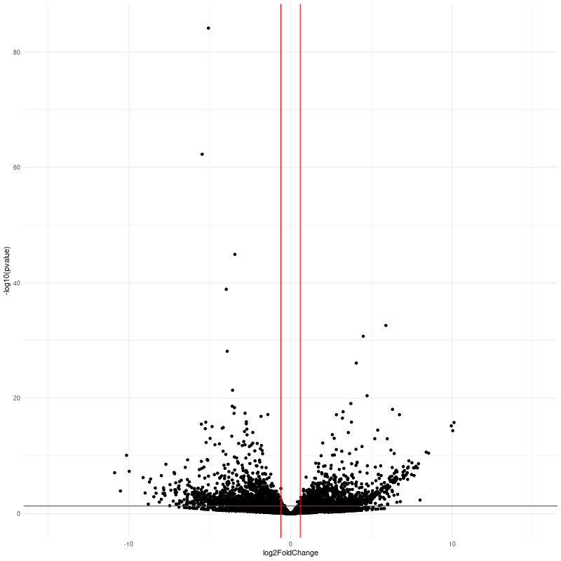 Identificar por colores los genes diferencialmente expresados ```r # Add a column to the data frame to specify if they are UP- or DOWN- regulated (log2FoldChange respectively positive or negative) de <- as.data.frame(res) # add a column of NAs de$diffexpressed <- "NO" # if log2Foldchange > 0.6 and pvalue < 0.05, set as "UP" de$diffexpressed[de$log2FoldChange > 0.6 & de$pvalue < 0.05] <- "UP" # if log2Foldchange < -0.6 and pvalue < 0.05, set as "DOWN" de$diffexpressed[de$log2FoldChange < -0.6 & de$pvalue < 0.05] <- "DOWN" png(file = paste0(outdir,"volcano04-res.png"), width = 800, height = 800) # guardar el plot en formato png *ggplot(data=de, aes(x=log2FoldChange, y=-log10(pvalue), col=diffexpressed)) + # cambiamos col param de aes geom_point() + theme_minimal() + geom_vline(xintercept=c(-0.6, 0.6), col="red") + geom_hline(yintercept=-log10(0.05), col="red") + xlim(-15,15) dev.off() ``` 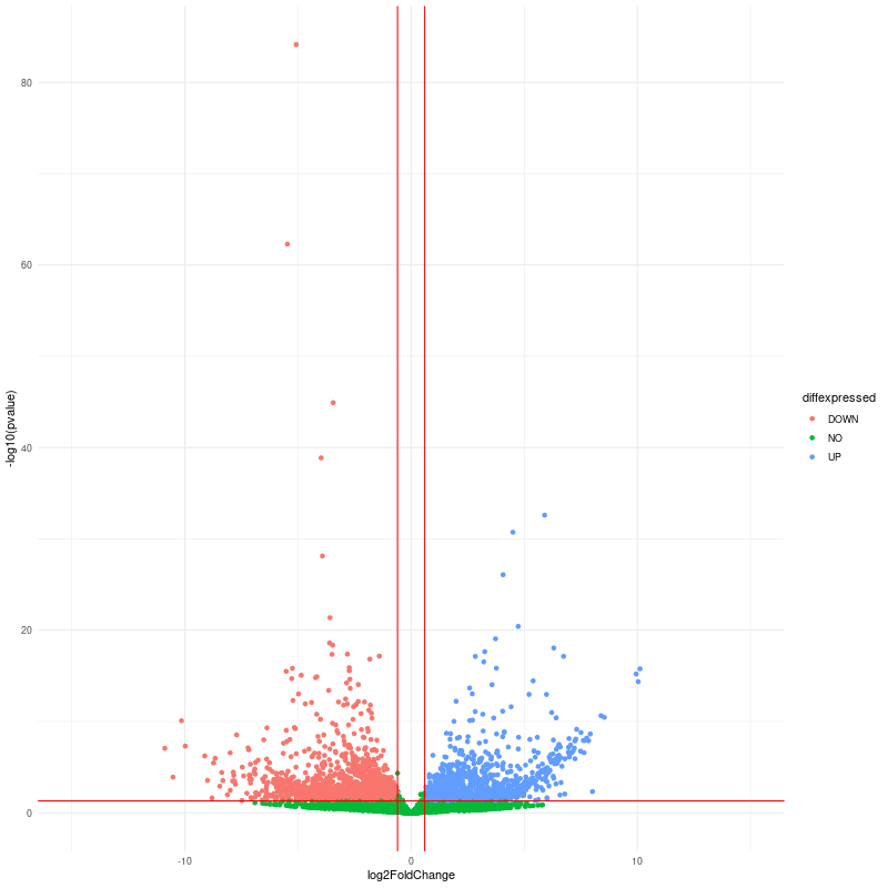 Cambiar colores de puntos, escribir nombres de genes ```r library(ggrepel) # libreria que evita el overlap de texto en labels # Create a new column "names" to de, that will contain the name of a subset if genes differentially expressed (NA in case they are not) de$names <- NA # filter for a subset of interesting genes *filter <- which(de$diffexpressed != "NO" & de$padj < 0.05 & (de$log2FoldChange >= 9 | de$log2FoldChange <= -9)) *de$names[filter] <- rownames(de)[filter] # Generar y guardara plot png(file = paste0(outdir,"volcano05-res.png"), width = 800, height = 800) # guardar el plot en formato png *ggplot(data=de, aes(x=log2FoldChange, y=-log10(pvalue), col=diffexpressed, label=names)) + geom_point() + * scale_color_manual(values=c("blue", "black", "red")) + # cambiar colores de puntos theme_minimal() + * geom_text_repel() + xlim(-15,15) dev.off() ``` 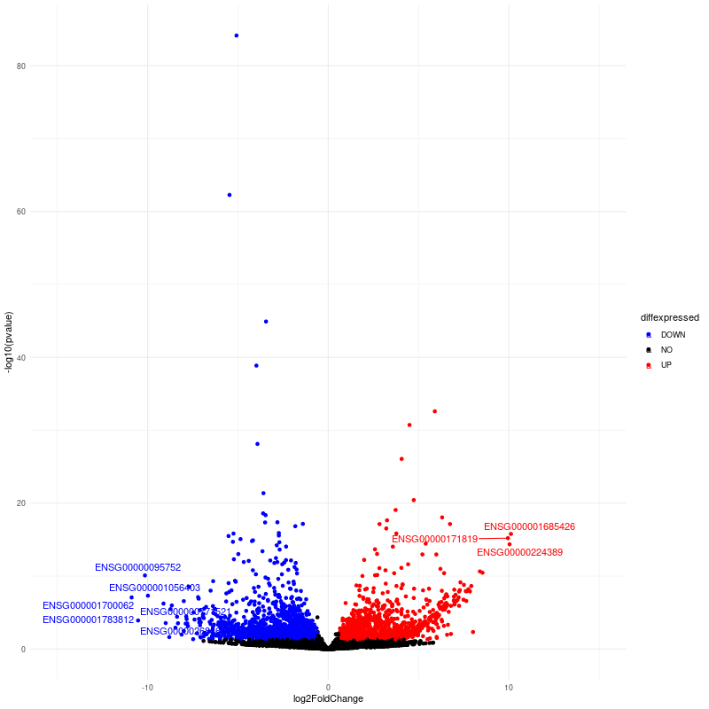 Practiquen cambiar otras cosas: labs, theme, titles, subtitles, colores de puntos, labels, etc. Ideas de edición: http://www.r-graph-gallery.com/index.html Referencia: https://biocorecrg.github.io/CRG_RIntroduction/volcano-plots.html ] --- # Heatmap - ¿Qué tipo de normalización deben tener los datos (cuentas) para visualizarlos en un heatmap? - .spoiler[vst() Para ajustar por la varianza de los genes, pues estaremos comparando genes y muestras] - [Referencia de imagen y código: sección 6.3](http://bioconductor.org/packages/release/workflows/vignettes/rnaseqGene/inst/doc/rnaseqGene.html) .fit[  ] --- # Enriquecimiento funcional de términos GO .scrollable[ - [gprofiler2](https://cran.r-project.org/web/packages/gprofiler2/vignettes/gprofiler2.html) - `gost` enables to perform functional profiling of gene lists. The function performs statistical enrichment analysis to find over-representation of functions from Gene Ontology, biological pathways like KEGG and Reactome, human disease annotations, etc. This is done with the hypergeometric test followed by correction for multiple testing. ```r library(gprofiler2) ``` ¿Cómo correr gost? [ver manual](https://cran.r-project.org/web/packages/gprofiler2/vignettes/gprofiler2.html) ```r # subset results for genes of interest resSig <- subset(res, padj < 0.1 & log2FoldChange > 1) # subset resSig <- resSig[ order(resSig$log2FoldChange, decreasing = TRUE), ] # define gene lists DEG <- rownames(resSig) *#genes_universe <- # enrichment analysis gostres = gost(query = DEG, organism = "hsapiens", significant = T, correction_method = "fdr", domain_scope = "custom", custom_bg = genes_universe, ordered_query = TRUE) names(gostres) attributes(gostres$meta) head(gostres$result) ``` ``` query significant p_value term_size query_size intersection_size 1 query_1 TRUE 4.892300e-03 3 9 3 2 query_1 TRUE 5.224098e-03 3 9 3 3 query_1 TRUE 4.963271e-05 11 205 9 4 query_1 TRUE 4.963271e-05 9 205 8 5 query_1 TRUE 5.373725e-05 12 205 10 6 query_1 TRUE 1.865613e-04 10 205 8 precision recall term_id source 1 0.33333333 1.0000000 GO:2000427 GO:BP 2 0.33333333 1.0000000 GO:2000425 GO:BP 3 0.04390244 0.8181818 HP:0000576 HP 4 0.03902439 0.8888889 HP:0001112 HP 5 0.04878049 0.8333333 HP:0001427 HP 6 0.03902439 0.8000000 HP:0000631 HP term_name effective_domain_size 1 positive regulation of apoptotic cell clearance 2676 2 regulation of apoptotic cell clearance 2676 3 Centrocecal scotoma 2676 4 Leber optic atrophy 2676 5 Mitochondrial inheritance 2676 6 Retinal arterial tortuosity 2676 source_order parents 1 29652 GO:0043277, GO:0050766, GO:2000425 2 29650 GO:0043277, GO:0050764 3 446 HP:0000575 4 874 HP:0000587 5 1073 HP:0000005 6 492 HP:0000630, HP:0005116, HP:0012841 ``` Generar Barplot ```r library(forcats) outdir = "/mnt/Citosina/amedina/mpadilla/clases/rnaseq/results/gost/" go <- as.data.frame(gostres$result) png(file = paste0(outdir,"gost01-resSig.png"), width = 800, height = 800) # guardar el plot en formato png # Reorder following the value of another column: go %>% arrange(p_value) %>% # order de acuerdo a valor incremental de pvalues select(term_name,p_value) %>% # seleccionar cols de df dplyr::slice(1:20) %>% # tomar las primeas 20 filas mutate(go = fct_reorder(term_name, p_value)) %>% ggplot( aes(x=go, y=p_value)) + geom_bar(stat="identity", fill="#3A68AE", alpha=.6, width=.4) + coord_flip() + labs(x = "", y = "Adjusted P-value") + theme_bw(base_size = 20) dev.off() ``` 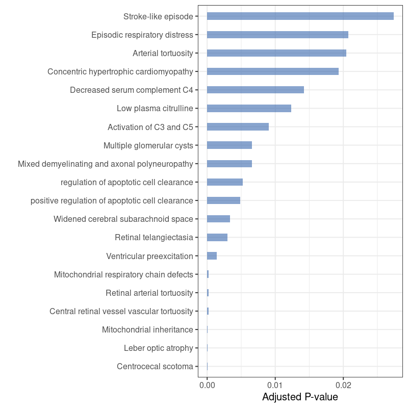 ] [kallisto]:https://pachterlab.github.io/kallisto/manual